Spectral Clustering

A tutorial on a simple version of the spectral clustering algorithm for clustering data points.

Spectral clustering is an important tool to seprate distinc section of data sets with complex structure. It works best on irregular data sets that simple clustering tools like sklearn.cluster.KMeans cannot identify.

To better compare what happen with clustering complex structure without spectral clustering, let’s look at an example where we use sklearn.cluster.KMeans, a simple clustering tool.

Simple Clustering Example:

import numpy as np
from sklearn import datasets
import matplotlib.pyplot as plt

n = 200
np.random.seed(1111)
X, y = datasets.make_blobs(n_samples=n, shuffle=True, random_state=None, centers = 2, cluster_std = 2.0)
plt.scatter(X[:,0], X[:,1])

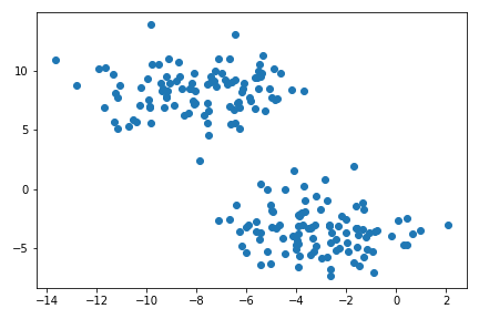
Clustering is an unsupervised learning problem. It refers to data analysis technique for discoviring patterns in data, organizing objects into groups whose members are similar in some way.

There are many algorithm for clusterin. A very common way for clustering is using KMeans, which has good performance on circular-ish blobs like these:

from sklearn.cluster import KMeans

km = KMeans(n_clusters = 2)
km.fit(X)

plt.scatter(X[:,0], X[:,1], c = km.predict(X))

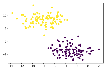
So for simple data blobs, KMeans clustering works fine. However, on a complex data structure, KMeans will perform badly.

np.random.seed(1234)
n = 200
X, y = datasets.make_moons(n_samples=n, shuffle=True, noise=0.05, random_state=None)
plt.scatter(X[:,0], X[:,1])

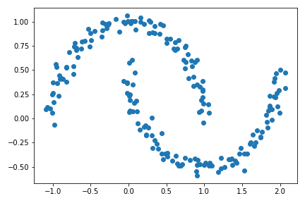
The structure now are crescents rather than blobs.

Matrix X contains the Euclidean coordinates of the data points.
Array y contains the labels of each point.

Since the irregular crescent structure, the simple circular clustering tool KMeans won’t work:

km = KMeans(n_clusters = 2)
km.fit(X)
plt.scatter(X[:,0], X[:,1], c = km.predict(X))

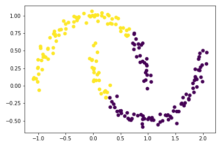
The graph above shows how badly KMeans performs on complex structure. For these situation, SPECTRAL CLUSTERING is a more appropriate tool.

Spectral Clustering Tutorial

NOTE: The Euclidean coordinates of the data points are contained in the matrix X, while the labels of each point are contained in y.

Notation:

Boldface capital letters like $\mathbf{A}$ = matrices (2d arrays of numbers).
Boldface lowercase letters like $\mathbf{v}$ = vectors (1d arrays of numbers).
$\mathbf{A}\mathbf{B}$ = matrix-matrix product (A@B).
$\mathbf{A}\mathbf{v}$ = matrix-vector product (A@v).

The overall maths:

Let $d_i = \sum_{j = 1}^n a_{ij}$ be the $i$th row-sum of $\mathbf{A}$, which is also called the degree of $i$.
Let $C_0$ and $C_1$ be two clusters of the data points. We assume that every data point is in either $C_0$ or $C_1$. The cluster membership as being specified by y. We think of y[i] as being the label of point i. So, if y[i] = 1, then point i (and therefore row $i$ of $\mathbf{A}$) is an element of cluster $C_1$.

\[N_{\mathbf{A}}(C_0, C_1)\equiv \mathbf{cut}(C_0, C_1)\left(\frac{1}{\mathbf{vol}(C_0)} + \frac{1}{\mathbf{vol}(C_1)}\right)\;.\]

In this expression,

$\mathbf{cut}(C_0, C_1) \equiv \sum_{i \in C_0, j \in C_1} a_{ij}$ is the cut of the clusters $C_0$ and $C_1$.
$\mathbf{vol}(C_0) \equiv \sum_{i \in C_0}d_i$, where $d_i = \sum_{j = 1}^n a_{ij}$ is the degree of row $i$ (the total number of all other rows related to row $i$ through $A$). The volume of cluster $C_0$ is a measure of the size of the cluster.

similarity matrix $\mathbf{A}$

$\mathbf{A}$ is a 2D np.ndarray matrix with shape (n, n) (n is the number of data points).
Entry A[i,j] should be equal to 1 if X[i] (the coordinates of data point i) is within distance epsilon of X[j] (the coordinates of data point j).
To get the distances, use sklearn.metrics.pairwise_distances on X coordinates. Also, set epsilon = 0.4 in this part
The diagonal entries A[i,i] equal to zero. Here we are using np.fill_diagonal()

from sklearn.metrics import pairwise_distances

# We have the Euclidean coordinate X, label y, with n = 200 above.
# Initiate our similarity matrix size nxn 
A = np.zeros((n,n)).astype(int)
epsilon = 0.4

# pairwise distances matrix from data X
distance_X = pairwise_distances(X)

# Entry A[i,j] = 1 if distance at corresponding distance_X is within epsilon
A[distance_X <= epsilon] = 1

# diagonal entries of A = 0
np.fill_diagonal(A,0)

# Check similarity matrix A
A

array([[0, 0, 0, ..., 0, 0, 0],
       [0, 0, 0, ..., 0, 0, 0],
       [0, 0, 0, ..., 0, 1, 0],
       ...,
       [0, 0, 0, ..., 0, 1, 1],
       [0, 0, 1, ..., 1, 0, 1],
       [0, 0, 0, ..., 1, 1, 0]])

Now we have a matrix that shows information of the pairwise distances between all points. label 1 means that the pairwise distance of the data points are close to each other within epsilon distance.

Cut Ojective

The cut term $\mathbf{cut}(C_0, C_1)$ is the number of nonzero entries in $\mathbf{A}$ that relate points in cluster $C_0$ to points in cluster $C_1$.

A small cut objective means points in $C_0$ is usually far from points in $C_1$.

cut(A,y) function compute the cut term by summing up the entries A[i,j] for each pair of points (i,j) in different clusters.

$\mathbf{cut}(C_0, C_1) \equiv \sum_{i \in C_0, j \in C_1} a_{ij}$ is the cut of the clusters $C_0$ and $C_1$.

def cut(A, y):
    # values in cluster 0:
    C0 = np.where(y == 0)[0]
    # values in cluster 1:
    C1 = np.where(y == 1)[0]

    # initiate sum for entries A[i,j] for each pair of points (i,j) in y
    cut_sum = 0
    for i in C0:
        for j in C1:
            cut_sum += A[i,j]
    # returns sum of points between 2 arrays associated to C0 and C1
    return cut_sum    

A reccomendation to make masks for clusters and iterating through each cluster values:

C_0_values = np.where(y == 0)[0] 
C_1_values = np.where(y == 1)[0]

Rather than check if i and j in range n belong to different cluster or not:

if y[i] != y[j]: cut_sum += A[i,j]

To better understand the cut objective value. We are going to compute the cut term for the true clusters y vs. a random vector of random labels y_random of length n with each label equal to either 0 or 1.

cut(A,y)

# random vector of random labels of length n
y_random = np.random.randint(2, size=n)
cut(A,y_random)

The cut terms reflect total points that are close together but got cut off into different cluster. So, if vector y puts points in matrix $\mathbf{A}$ that are close together into different clusters, the cut term will increase. Our target is to minimize this cut terms to better distinguished between spectral clusters.

y_random is randomly assigning labels to points in $\mathbf{A}$, resulting in very high cut number. Compare to this random set, the cut objective for the true labels of 26 is much smaller, indicating the cut term indeed favors the true clusters over the random ones.

Volume Objective

The second factor in the binary norm cut objective: volume term.
Volume of cluster measures how big the cluster is.
If cluster $C_0$ is small, then $\mathbf{vol}(C_0)$ will be small and $\frac{1}{\mathbf{vol}(C_0)}$ will be large, leading to an undesirable higher objective value.

Function vols(A,y) computes the volumes of $C_0$ and $C_1$, returning them as a tuple. For example, v0, v1 = vols(A,y) should result in v0 holding the volume of cluster 0 and v1 holding the volume of cluster 1.

$\mathbf{vol}(C_0) \equiv \sum_{i \in C_0}d_i$, where $d_i = \sum_{j = 1}^n a_{ij}$ is the degree of row $i$ (the total number of all other rows related to row $i$ through $A$). The volume of cluster $C_0$ is a measure of the size of the cluster.

def vols(A,y):
    # vols C0 == 𝑖 th row-sum of 𝐀, y label 0, C1 label 1
    vol_C0 = A[y==0,:].sum()
    vol_C1 = A[y==1,:].sum()
    return (vol_C0, vol_C1)

Binary Normcut Objective

The binary normcut objective purpose is to find clusters $C_0$ and $C_1$ such that:

There are relatively few entries of $\mathbf{A}$ that join $C_0$ and $C_1$.
Neither $C_0$ and $C_1$ are too small.

Applying the formula: $N_{\mathbf{A}}(C_0, C_1)\equiv \mathbf{cut}(C_0, C_1)\left(\frac{1}{\mathbf{vol}(C_0)} + \frac{1}{\mathbf{vol}(C_1)}\right)\;$

def normcut(A,y):
    c = cut(A,y)
    v0, v1 = vols(A,y)
    return c * (1/v0 + 1/v1)

Compare the normcut objective using both the true labels y and the fake labels y_random generated above:

print("true labels: ", normcut(A,y))
print("Random labels", normcut(A,y_random))

true labels:  0.02303682466323045
Random labels 2.0650268054241563

The normcut true label cluster is much smaller than the randomized label. Hence, y label of clusters $C_0, C_1$ is a good partition of data since $N_{\mathbf{A}}(C_0, C_1)$ normcut metric is small.

Alternative Expression for Normcut Objective

Define a new vector $\mathbf{z} \in \mathbb{R}^n$ whereL

\[z_i = \begin{cases} \frac{1}{\mathbf{vol}(C_0)} &\quad \text{if } y_i = 0 \\ -\frac{1}{\mathbf{vol}(C_1)} &\quad \text{if } y_i = 1 \\ \end{cases}\]

The signs of the elements of $\mathbf{z}$ contain information from $\mathbf{y}$: if $i$ is in cluster $C_0$, then $y_i = 0$ and $z_i > 0$.

Then, proves that the normalized cut objective is the same as this equation:

\[\mathbf{N}_{\mathbf{A}}(C_0, C_1) = 2\frac{\mathbf{z}^T (\mathbf{D} - \mathbf{A})\mathbf{z}}{\mathbf{z}^T\mathbf{D}\mathbf{z}}\;,\]

where $\mathbf{D}$ is the diagonal matrix with nonzero entries $d_{ii} = d_i$, and where $d_i = \sum_{j = 1}^n a_i$ is the degree (row-sum) from before.

Tasks:

transform(A,y) function computes the appropriate $\mathbf{z}$ vector given A and y, using the formula above.
Check the equation above that relates the matrix product to the normcut objective, by computing each side separately and checking that they are equal.
Check the identity $\mathbf{z}^T\mathbf{D}\mathbb{1} = 0$, where $\mathbb{1}$ is the vector of n ones (i.e. np.ones(n)). This identity effectively says that $\mathbf{z}$ should contain roughly as many positive as negative entries.

Transform(A,y)

def transform(A,y):
    v0, v1 = vols(A,y)
    # using the formular for z, set all z values to 1/vol(C0) first
    z = np.full(n, 1/v0)
    
    # then seek out label y=1 and reset the value of z to -1/vol(C1)
    z[y==1] = -1/v1
    
    return z

The code vols(A,y) was told to be concise and helpful. The transform(A,y) function, the use of np.full is said to be a clever way to set the size of the vector (no need to create an empty vector, then filled in for 1 and 0 separately).

Check the normcut objective

# compute D diagonal matrix with nonzero entries dii = di, di = row-sum
D = np.diag(A.sum(axis = 1))

z = transform(A,y)

# check both normcut objectives:
norm1 = normcut(A,y)
norm2 = 2 * (z@(D-A)@z) / (z@D@z)

norm1, norm2

(0.02303682466323045, 0.023036824663230267)

Compare the 2 normcut computations by using np.isclose(a,b) (due to computer arithmetic limitation, the numbers are not exactly the same)

np.isclose(norm1, norm2)

True

Check the identity $\mathbf{z}^T\mathbf{D}\mathbb{1} = 0$

z@D@np.ones(n), np.isclose(z@D@np.ones(n), 0)

(-4.5102810375396984e-17, True)

This identity effectively proves that $\mathbf{z}$ contain roughly as many positive as negative entries.

Orthogonal Objective Optimization: `scipy.optimize.minimize` method

Since we have the alternative expression for constructing normalized cut objective, we can perform optimization normcut objective by minimizing the function:

\[R_\mathbf{A}(\mathbf{z})\equiv \frac{\mathbf{z}^T (\mathbf{D} - \mathbf{A})\mathbf{z}}{\mathbf{z}^T\mathbf{D}\mathbf{z}}\]

subject to the condition $\mathbf{z}^T\mathbf{D}\mathbb{1} = 0$.

To embedded this condition, substituting $\mathbf{z}$ the orthogonal complement of $\mathbf{z}$ relative to $\mathbf{D}\mathbf{1}$.

Referencing professor Philips Chodrow for the code below, with orth_obj function and using the minimize function from scipy.optimize to minimize the function orth_obj with respect to $\mathbf{z}$.

def orth(u, v):
    return (u @ v) / (v @ v)*v

e = np.ones(n) 

d = D @ e

def orth_obj(z):
    z_o = z - orth(z, d)
    return (z_o @ (D - A) @ z_o)/(z_o @ D @ z_o)

from scipy.optimize import minimize
# minimize vector z_
z_min = minimize(orth_obj, z)

Visualize clusters

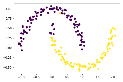
The minimize() function above gave an approximately optimizing for the normcut objective (continuous relaxation of the normcut problem),

Due to the approximation, We gonna use -0.0015 instead of 0 to differentiate between the negative and positive values (this is a trials and errors thing, -0.0015 works best out of all 0 approximation)

plt.scatter(X[:,0], X[:,1], c = z_min.x < -0.0015)

)

Although close, but there are still mistakenly label data points for this optimization using minimize() method.

Improved Objective Optimization: Eigenvectors method

Rewind back to the function used for minimizing: $R_\mathbf{A}(\mathbf{z})\equiv \frac{\mathbf{z}^T (\mathbf{D} - \mathbf{A})\mathbf{z}}{\mathbf{z}^T\mathbf{D}\mathbf{z}}$

with respect to $\mathbf{z}$, subject to the condition $\mathbf{z}^T\mathbf{D}\mathbb{1} = 0$.

According to the Rayleigh-Ritz Theorem,minimizing $\mathbf{z}$ is solved by finding the smallest eigenvalue of the generalized eigenvalue problem

\[(\mathbf{D} - \mathbf{A}) \mathbf{z} = \lambda \mathbf{D}\mathbf{z}\;, \quad \mathbf{z}^T\mathbf{D}\mathbb{1} = 0\]

which is equivalent to the standard eigenvalue problem

\[\mathbf{D}^{-1}(\mathbf{D} - \mathbf{A}) \mathbf{z} = \lambda \mathbf{z}\;, \quad \mathbf{z}^T\mathbb{1} = 0\;.\]

Since $\mathbb{1}$ is actually the eigenvector with smallest eigenvalue of the matrix $\mathbf{D}^{-1}(\mathbf{D} - \mathbf{A})$, the vector $\mathbf{z}$ that we want must be the eigenvector with the second-smallest eigenvalue.

Tasks:

Construct the matrix $\mathbf{L} = \mathbf{D}^{-1}(\mathbf{D} - \mathbf{A})$, which is often called the Laplacian matrix of the similarity matrix $\mathbf{A}$.
Find the eigenvector corresponding to its second-smallest eigenvalue, and call it z_eig.
plot the data again, using the sign of z_eig as the color.

# construct Laplacian matrix
L = np.linalg.inv(D)@(D-A)

# eigenvalue and eigenvector
eigval, eigvec = np.linalg.eig(L)

# argsort eigenvector and correspond eigenvalue from smallest to largest
ix = eigval.argsort()
eigval, eigvec = eigval[ix], eigvec[:,ix]

# second-smallest correspond unit eigenvector
z_eig = eigvec[:,1]

# plot result
plt.scatter(X[:,0], X[:,1], c = z_eig < 0)

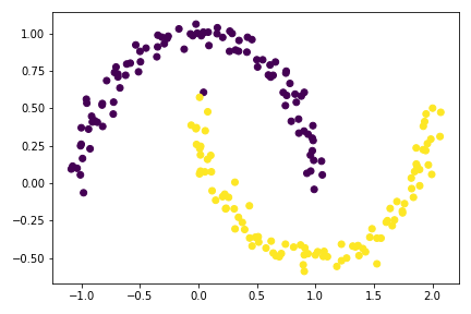
Previously, I accidently use (L+ L.T)/2 in np.linalg.eig(), a friendly peer pointed out that since the Laplacian matrix is already a nonsingular square matrix, we can directly find the eigenvalues and eigenvectors using L itself.

The result plot is much better than the z_min method, although it is not perfect due to limit precision of minimization by default.

Compact function for Spectral Clustering Algorithm

A combination of everything we went throught so far, minusing the unsuccessful one and go straight out to the best algorithm only!

Function spectral_clustering(X, epsilon), which takes in the input data X and the distance threshold epsilon and performs spectral clustering, returning an array of binary labels indicating whether data point i is in group 0 or group 1.

Outline

Construct the similarity matrix.
Construct the Laplacian matrix.
Compute the eigenvector with second-smallest eigenvalue of the Laplacian matrix.
Return labels based on this eigenvector.

def spectral_clustering(X, epsilon):
    """
    Performes spectral clustering
    argument:
        X: matrix contain Euclidean coordinates of the data points
        epsilon: distance threshold
    Return:
        an array of binary labels indicating whether data point i is in group 0 or 1.
    """
    
    # construct similarity matrix:
    A = np.zeros((n,n))
    A[pairwise_distances(X) <= epsilon] = 1
    np.fill_diagonal(A,0)
    
    # construct Laplacian matrix:
    D = np.diag(A.sum(axis = 1))
    L = np.linalg.inv(D) @ (D-A)
    
    # compute eigenvector with second-smallest eigenvalue of laplacian matrix:
    eigval, eigvec = np.linalg.eig((L + L.T)/2)
    eigvec = eigvec[:, eigval.argsort()]
    z_eig = eigvec[:,1]
    
    # return labels based on this eigenvector
    return (eigvec[:,1] <0).astype(int)

A comments was made about how efficient it is using eigvec = eigvec[:, eigval.argsort()] and return (eigvec[:,1] <0).astype(int)

# plot result
plt.scatter(X[:,0], X[:,1], c = spectral_clustering(X, 0.4))

Examples using `spectral_clustering` function

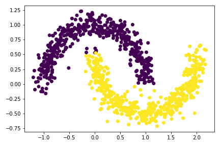
Experiment with `make_moons` datasets. Change `noise` setting:

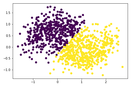
The noise parameters often causes the algorithms to miss out patterns in the data, so here, we want to see how is this parameter will affects the accuracy of our spectral clustering algorithm

np.random.seed(1234)
n = 1000
X, y = datasets.make_moons(n_samples=n, shuffle=True, noise=0.1, random_state=None)
plt.scatter(X[:,0], X[:,1], c = spectral_clustering(X, 0.4))

np.random.seed(1234)
n = 1000
X, y = datasets.make_moons(n_samples=n, shuffle=True, noise=0.3, random_state=None)
plt.scatter(X[:,0], X[:,1], c = spectral_clustering(X, 0.7))

Add annotation to the experiments with noises:
Increasing noise would affect the algorigthm. At noise=0.3, the data sets now looks like a single big blobs with no distinctive pattern. Hence, the algorithm splits the blobs in half.

Thanks y’all! I appreciate all the helps I received.

Experiment with `make_circles()` – the bull’s eye data set:

n = 1000
X, y = datasets.make_circles(n_samples=n, shuffle=True, noise=0.05, random_state=None, factor = 0.4)
plt.scatter(X[:,0], X[:,1])

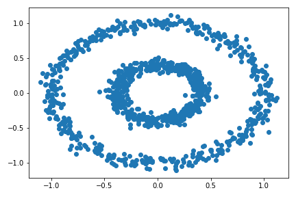
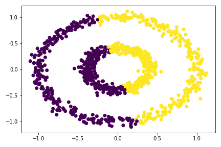
There are two concentric circles. As before k-means will not do well here at all.

km = KMeans(n_clusters = 2)
km.fit(X)
plt.scatter(X[:,0], X[:,1], c = km.predict(X))

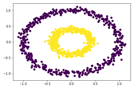
# apply the spectral_clustering() function
plt.scatter(X[:,0], X[:,1], c = spectral_clustering(X, 0.4))

plt.scatter(X[:,0], X[:,1], c = spectral_clustering(X, 0.33))

plt.scatter(X[:,0], X[:,1], c = spectral_clustering(X, 0.3))

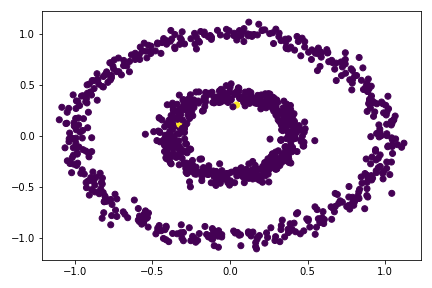
plt.scatter(X[:,0], X[:,1], c = spectral_clustering(X, 0.5))

plt.scatter(X[:,0], X[:,1], c = spectral_clustering(X, 0.53))

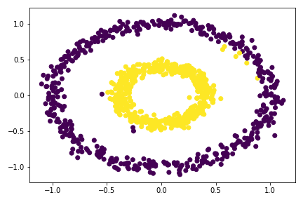
So I tried multiple epsilon here, from 0.3 to 0.55, the best value is around 0.33 - 0.53. For epsilon 0.53, there is already mis-categorize data points. Going out of this range would cause the clustering failed completely.

Written on April 30, 2021

PIC 16B Blog

Spectral Clustering

Simple Clustering Example:

Spectral Clustering Tutorial

The overall maths:

similarity matrix \(\mathbf{A}\)

Cut Ojective

Volume Objective

Binary Normcut Objective

Alternative Expression for Normcut Objective

Transform(A,y)

Check the normcut objective

Check the identity \(\mathbf{z}^T\mathbf{D}\mathbb{1} = 0\)

Orthogonal Objective Optimization: `scipy.optimize.minimize` method

Visualize clusters

Improved Objective Optimization: Eigenvectors method

Compact function for Spectral Clustering Algorithm

Outline

Examples using `spectral_clustering` function

Experiment with `make_moons` datasets. Change `noise` setting:

Experiment with `make_circles()` – the bull’s eye data set:

Spectral Clustering

Simple Clustering Example:

Spectral Clustering Tutorial

The overall maths:

similarity matrix \(\mathbf{A}\)

Cut Ojective

Volume Objective

Binary Normcut Objective

Alternative Expression for Normcut Objective

Transform(A,y)

Check the normcut objective

Check the identity \(\mathbf{z}^T\mathbf{D}\mathbb{1} = 0\)

Orthogonal Objective Optimization: scipy.optimize.minimize method

Visualize clusters

Improved Objective Optimization: Eigenvectors method

Compact function for Spectral Clustering Algorithm

Outline

Examples using spectral_clustering function

Experiment with make_moons datasets. Change noise setting:

Experiment with make_circles() – the bull’s eye data set:

Orthogonal Objective Optimization: `scipy.optimize.minimize` method

Examples using `spectral_clustering` function

Experiment with `make_moons` datasets. Change `noise` setting:

Experiment with `make_circles()` – the bull’s eye data set: